Chapter 2 Nuclear Stability and the Liquid Drop Model

2.1 Introduction

In lecture 1 we saw that most nuclides are unstable and there is just a small “island” of stability in $N$ and $Z$ which is illustrated by the Segre Chart. How can this be explained?

2.2 Nuclear binding energy

A nucleus has less mass than the sum of its individual nucleons. You can think of the binding energy of a nucleus as the energy released when the constituent protons and neutrons are brought together. You can also think of the binding energy as the energy required to separate a nucleus into its constituent protons and neutrons.

The difference in mass between the nucleus and its constituent protons and neutrons is called the mass defect. The higher the mass defect, the greater the energy release when constituent nucleons are brought together/the greater the energy required to separate nucleus into constituent nucleons.

Data sources (books, websites, exams!) usually provide atomic masses, but not always. To obtain nuclear masses from atomic masses we need to subtract the masses of the electrons for a given atom. We should also include the binding energy of the electrons, but this term is usually negligible compared to the binding energy of the nucleus:

$$M_N{c}^2=M_A{c}^2-Z{m}_e{c}^2+\sum _i^Z{B}_i,$$ (2.1)

where $M_N$ is the nuclear mass, $M_A$ the atomic mass, $m_e$ the mass of the electron and $B_i$ the binding energy of the $i^{th}$ electron. Electronic binding energies are typically $10-100$ keV whereas atomic masses correspond to energies of order $A\times$1000 MeV, so it is usual to neglect the former.

The nuclear binding energy $B$ is then given by:

$$B=\{Z{m}_p+N{m}_n-M_N{(}^A\mathrm{X})\}{c}^2.$$ (2.2)

or in terms of the atomic mass

$$B=\{Z{m}_p+N{m}_n-[M_A{(}^A\mathrm{X})-Z{m}_e]\}{c}^2.$$ (2.3)

Note that we can re-write this in the form:

$$B=\{N{m}_n+Z{M}_A{(}^1\mathrm{H})-M_A{(}^A\mathrm{X})\}{c}^2,$$ (2.4)

which can be slightly easier to handle when making calculations if you have atomic masses available.

Careful 2.2.1.

Check what type of mass you are given in a question. Typically they will be atomic masses, but not always.

Example 2.2.1 (Energy Release).

Derive an expression for the energy release, $Q$, in terms of the binding energy of the parent nucleus, $X$, and daughter nucleus, $Y$, when $X$ decays via ${\beta }^{-}$ emission.

Solution.

The decay process is

$$X\to Y+e^{-}+{\overline{\nu }}_e.$$

The general expression for $Q$ is

$$Q=\left[\sum M_N{(A,Z)}_{reactants}-\sum M_N{(A,Z)}_{products}\right]c^2,$$

which for ${\beta }^{-}$ emission gives

$$Q=\left[M_N(A,Z)-M_N(A,Z+1)-m_e\right]c^2.$$

The general expression for $B$ is

$$B(A,Z)=\left[Z{m}_p+(A-Z)m_n-M_N(A,Z)\right]c^2,$$

which on rearranging for $M_N$ gives

$$M_N(A,Z)=Z{m}_p+(A-Z)m_n-B(A,Z)/c^2.$$

This can be substituted into the expression for $Q$ for ${\beta }^{-}$ emission

$$Q=\left[m_n-m_p-m_e\right]c^2+B(A,Z+1)-B(A,Z).$$

The masses are $m_p=938.272\mathrm{MeV}/c^2$, $m_n=939.565\mathrm{MeV}/c^2$ and $m_e=0.511\mathrm{MeV}/c^2$. This gives the term $\left[m_n-m_p-m_e\right]c^2=0.782\mathrm{MeV}$.

To calculate $Q$, we would then need the binding energies, using either exact values or approximations from the semi-empirical binding energy formula. ∎

We will now perform two examples of writing the energy release, $Q$, in terms of the binding energies.

Example 2.2.2 (Energy Release).

Repeat the previous example when $X$ decays via ${\beta }^{+}$ emission.

Solution.

The decay process is

$$X\to Y+e^{+}+{\nu }_e.$$

The general expression for $Q$ is

$$Q=\left[\sum M_N{(A,Z)}_{reactants}-\sum M_N{(A,Z)}_{products}\right]c^2,$$

which for ${\beta }^{+}$ emission gives

$$Q=\left[M_N(A,Z)-M_N(A,Z-1)-m_e\right]c^2.$$

The general expression for $B$ is

$$B(A,Z)=\left[Z{m}_p+(A-Z)m_n-M_N(A,Z)\right]c^2,$$

which on rearranging for $M_N$ gives

$$M_N(A,Z)=Z{m}_p+(A-Z)m_n-B(A,Z)/c^2.$$

This can be substituted into the expression for $Q$ for ${\beta }^{+}$ emission

$$Q=\left[m_p-m_n-m_e\right]c^2+B(A,Z-1)-B(A,Z).$$

The masses are $m_p=938.272\mathrm{MeV}/c^2$, $m_n=939.565\mathrm{MeV}/c^2$ and $m_e=0.511\mathrm{MeV}/c^2$. This gives the term $\left[m_p-m_n-m_e\right]c^2=-1.804\mathrm{MeV}$.

To calculate $Q$, we would then need the binding energies, using either exact values or approximations from the semi-empirical binding energy formula. ∎

2.2.1 Binding energy per nucleon

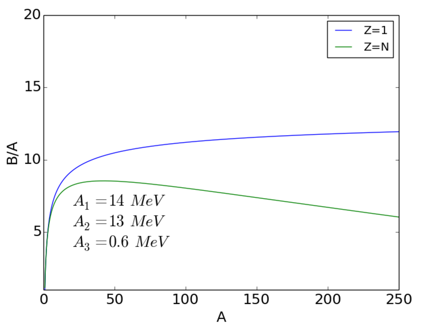
From Eqns. (2.3) and (2.4) we can easily calculate the binding energy per nucleon ($B/A$) and plot this against mass number $A$, as shown in Fig. 2.1.

Example 2.2.3 (Binding Energy Per Nucleon).

The mass of a neutron and proton are $1.00866\mathrm{u}$ and $1.00728\mathrm{u}$ respectively, where 1 atomic mass unit (u) is $931.5\mathrm{MeV}/{\mathrm{c}}^2$. The nuclear mass of an alpha particle is $4.00153\mathrm{u}$. The mass defect is then $2\times 1.00866\mathrm{u}+2\times 1.00728\mathrm{u}-4.00153\mathrm{u}=0.03035\mathrm{u}=28.3\mathrm{MeV}/{\mathrm{c}}^2$. Converting this to energy by multiplying by $c^2$, the binding energy is 28.3 MeV, or 7.1 MeV per nucleon.

Figure 2.1: The binding energy per nucleon ($B/A$) versus mass number $A$ for stable nuclei.

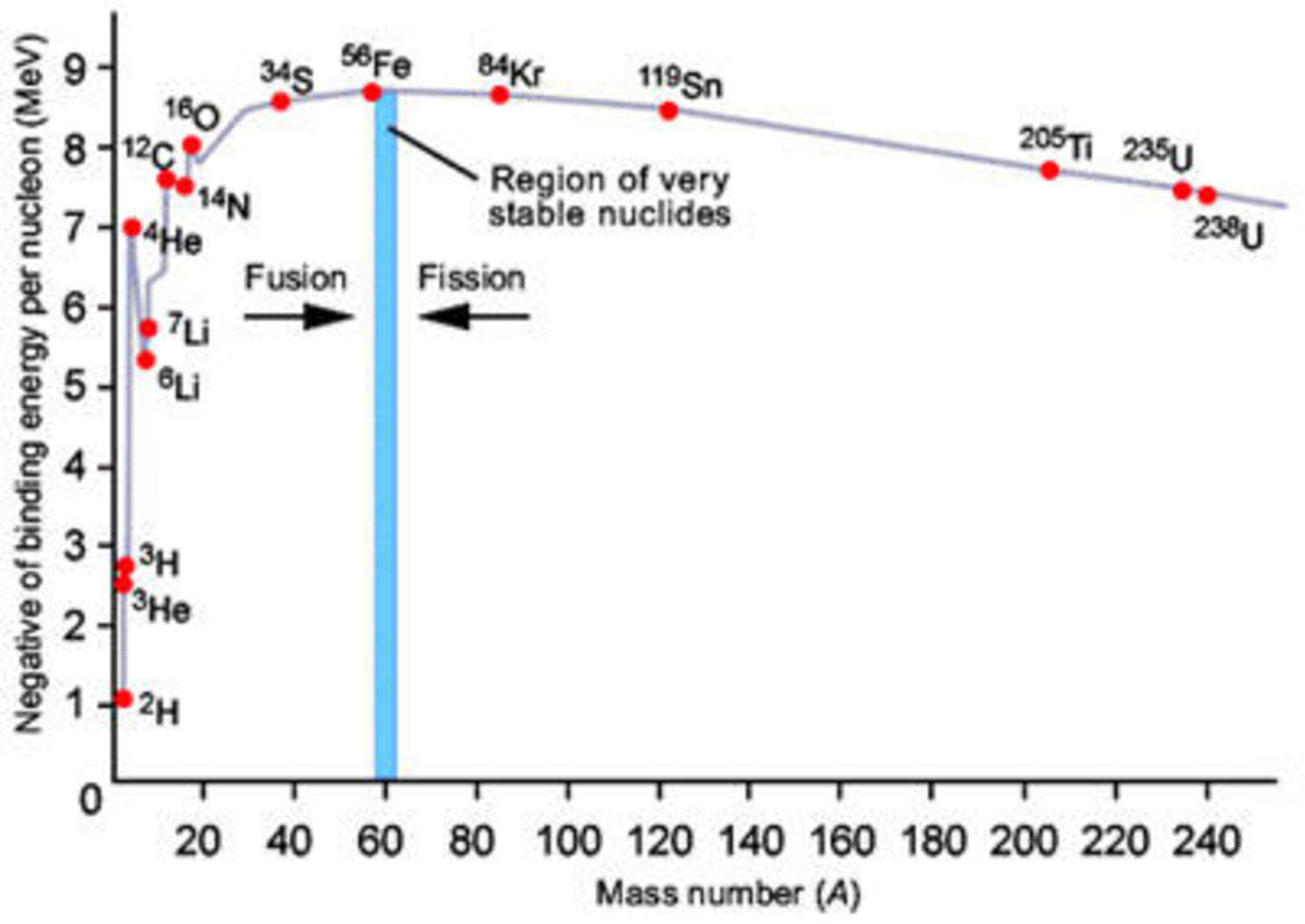
We note that the curve reaches a maximum near $A=60$, where the nucleons are most tightly bound. This suggests that we can release this binding energy in one of two ways. For we can assemble lighter nuclei into heavier nuclei and for $A>60$ we can break heavier nuclei into lighter nuclei. These processes are known, respectively, as nuclear fusion and nuclear fission. We will discuss them in greater detail later. The other remarkable feature is that for $A>16$ the binding energy per nucleon is within 10% of 8 MeV.

2.3 Nuclear diameters

If we imagine individual nucleons as spheres with radius $R_0$, then the total volume of a nucleus is $A\times 4\pi R_0^3/3$, since the mass number $A$ is the number of nucleons. If the nucleus has radius $R$, we can equate $4\pi R^3/3=A\mathrm{\hspace{0.17em}4}\pi R_0^3/3$, giving $R=R_0{A}^{1/3}$. $R_0$ is a constant to be found experimentally. A typical value is $R_0=1.2\times {10}^{-15}\mathrm{m}$, although this will vary depending on the experiment.

2.4 The semi-empirical binding energy formula

The simplest physically useful model of the nucleus was proposed by von Weizacker in 1935. It treats the nucleus as a drop of incompressible fluid.

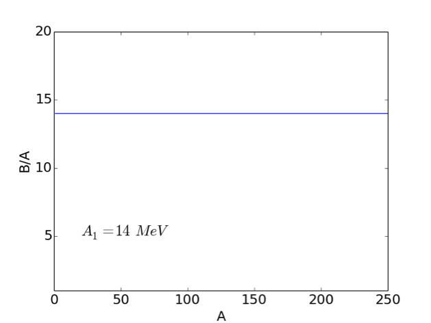
The observation that, for all but the lightest nuclei, the binding energy per nucleon is roughly constant (i.e. $B/A\sim \mathrm{const}$ ), suggests that we can assume that $B\propto A$. This simple mathematical statement has important physical implications. For example, consider a situation in which each nucleon had an attractive interaction with all the other nucleons in the nucleus. In this case, we would find that:

$$B\propto A(A-1)\propto A^2.$$ (2.5)

Difficult 2.4.1.

The $A(A-1)$ and $Z(Z-1)$ terms count the total number of nucleon and proton pairs respectively. There are $A(A-1)/2$ and $Z(Z-1)/2$ independent pairs (i.e. avoiding double counting).

Volume term

Our observation that $B\propto A$ indicates that nucleons only interact with their nearest neighbours. In other words, the strong nuclear force that holds nuclei together is very short-range. If we imagine our nucleus is a drop of fluid in which each nucleon interacts only with its nearest neighbours, we can define a volume energy

$$B_{\mathrm{v}}=a_{1}A.$$ (2.6)

This term is shown in Fig. 2.2.

Figure 2.2: The volume contribution to $B/A$.

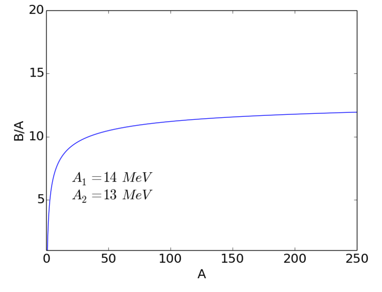
Surface term

However, some nucleons are on the surface of the nucleus and thus have fewer neighbours, hence smaller binding energy. We need to correct for this.

The nuclear radius is given by

$R$ $=$ $R_0{A}^{1/3}.$ (2.7)

The surface area of the nucleus is then

$$4\pi R^2=4\pi R_0^2{A}^{2/3}.$$ (2.8)

The binding energy of the nucleus is therefore reduced by the presence of the surface by

$$B_{\mathrm{s}}=-a_2{A}^{2/3}.$$ (2.9)

The surface energy term is analogous to the surface tension in a liquid drop. The combined volume + surface terms are shown in Fig. 2.3.

Figure 2.3: The volume and surface contributions to $B/A$.

Coulomb term

Some of the nucleons in our liquid drop are protons, carrying a positive charge. They therefore suffer a repulsive Coulomb interaction $B_{\mathrm{c}}$. There are $Z(Z-1)/2$ pairs of protons in a nucleus of atomic number $Z$. (The factor of 1/2 prevents double counting). Each pair interacts by a Coulomb repulsion giving a negative contribution to the binding energy

$$B_{\mathrm{c}}=-\frac{Z(Z-1)e^2}{8\pi {ϵ}_0{r}_{\mathrm{av}}},$$ (2.10)

where $r_{\mathrm{av}}$ is the average separation of the protons. To first order

$$r_{\mathrm{av}}\propto R\propto A^{1/3}.$$ (2.11)

We can therefore write

$$B_{\mathrm{c}}=-a_{3}Z(Z-1)A^{-1/3}.$$ (2.12)

So far we have three terms in our model, which can be understood by considering a charged incompressible drop of liquid. Putting them together, we have

$$B=a_{1}A-a_2{A}^{2/3}-a_{3}Z(Z-1)A^{-1/3}.$$ (2.13)

If this were the complete expression for the nuclear binding energy, the most stable nucleus would have $Z=1$ and $N(=A-Z)$ infinite! The combined volume + surface + Coulomb terms are shown in Fig. 2.4.

Figure 2.4: The volume, surface and Coulomb contributions to $B/A$.

Asymmetry term

Clearly, we don’t find isotopes of hydrogen $(Z=1)$ with arbitrarily large numbers of neutrons, so our description so far is incomplete. Recall that the Segre chart shows that $N=Z$ is favoured, especially for light nuclei. For our model to fit the data, we need to introduce a term that will ‘encourage’ nuclei to have $N\simeq Z$ and which becomes less significant with increasing $A$. This term is the asymmetry energy

$$B_{\mathrm{a}}=-a_4\frac{{(A-2Z)}^2}{A}.$$ (2.14)

The combined volume + surface + Coulomb + asymmetry terms are shown in Fig. 2.5.

Figure 2.5: The volume, surface, Coulomb and asymmetry contributions to $B/A$.

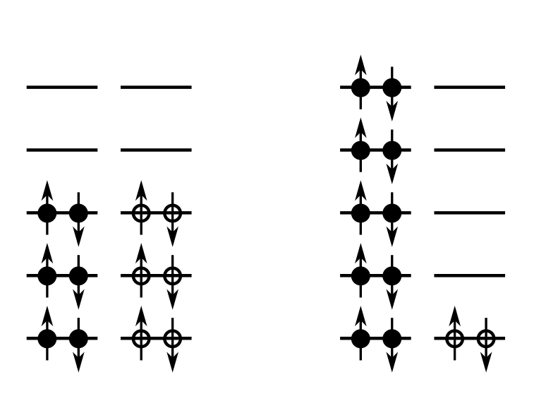
There is in fact a physical origin for the asymmetry term. We need to consider the nucleons as occupying energy levels in a potential well. (We will look at this in greater detail next lecture when we consider the shell model of the nucleus). Protons and neutrons are fermions (spin 1/2) which means they obey the Pauli exclusion principle – only two particles of each type, with spin “up” and spin “down” can occupy a given energy level, as illustrated in Fig. 2.6.

Figure 2.6: Schematic nucleon energy levels.

To create a neutron excess without changing $A$ we can convert two proton pairs into two neutron pairs (a thought experiment), as shown in Fig. 2.7.

Figure 2.7: Energy levels resulting from the conversion of two pairs of protons to neutrons.

If the spacing between energy levels is $ϵ$, then each ‘new’ neutron pair has $2ϵ$ greater energy than the proton pair from which it was “created”. Therefore the energy difference between isobars is given by:

$\mathrm{\Delta }E=$ $\mathrm{number}\mathrm{of}\mathrm{new}\mathrm{neutrons}\times \mathrm{energy}\mathrm{increase}\mathrm{per}\mathrm{neutron},$

$\mathrm{\Delta }E=$ $\left[{\displaystyle \frac{1}{2}}(N-Z)\right]\times \left[{\displaystyle \frac{1}{2}}(N-Z){\displaystyle \frac{ϵ}{2}}\right]$

$=$ ${\displaystyle \frac{ϵ}{8}}{(N-Z)}^2.$ (2.15)

The asymmetry contribution to the binding energy, $B_{\mathrm{a}}$, is therefore:

$$B_{\mathrm{a}}\propto {(N-Z)}^2.$$ (2.16)

The energy level spacing varies as $A^{-1}$ so we have

$$B_{\mathrm{a}}\propto \frac{{(N-Z)}^2}{A}.$$ (2.17)

Pairing term

There is one final term needed for the model to fit reality – the pairing energy term. From the Segre Chart we see that nuclei with pairs of protons and neutrons, i.e. even $N$ and/or even $Z$, are the most stable. Only 4 stable odd $N$, odd $Z$ nuclides exist. We can also see that the pairing of nuclei is less important for heavier nuclei. We introduce a pairing energy term

$$B_{\mathrm{p}}=(\pm ,0)\frac{a_5}{A^{3/4}},$$ (2.18)

where $B_{\mathrm{p}}$ = positive for even-even nuclei, 0 for even-odd and odd-even nuclei, and negative for odd-odd nuclei.

Difficult 2.4.2.

Be sure you are familiar with the $(\pm ,0)$ notation for the pairing term. This means: $+$ for even $Z$, even $N$; $0$ for even $Z$, odd $N$; $0$ for odd $Z$, even $N$; $-$ for odd $Z$, odd $N$.

Putting all the terms together we obtain the semi-empirical binding energy formula:

$$B=a_{1}A-a_2{A}^{2/3}-a_{3}Z(Z-1)A^{-1/3}-a_4\frac{{(A-2Z)}^2}{A}+(\pm ,0)\frac{a_5}{A^{3/4}}.$$ (2.19)

The coefficients $a_i$ are found by fitting the experimental binding energy curve. Typical values are

$a_1$ $=$ $14\mathrm{MeV},$ (2.20)

$a_2$ $=$ $13\mathrm{MeV},$

$a_3$ $=$ $0.6\mathrm{MeV},$

$a_4$ $=$ $19\mathrm{MeV},$

$a_5$ $=$ $34\mathrm{MeV}.$

The combined volume + surface + Coulomb + asymmetry + pairing terms are shown in Fig. 2.8.

Figure 2.8: The volume, surface, Coulomb, asymmetry, and pairing contributions to $B/A$.

Example 2.4.1 (Nuclear Stability).

Calculate the binding energy per nucleon of ${}_{20}{}^{}{}_{}{}^{40}$Ca. Compare this to the value predicted by the semi-empirical binding energy. The atomic masses are $M_A{(}^1\mathrm{H})=1.00783\mathrm{u}$ and $M_A{(}^{40}\mathrm{Ca})=39.96259\mathrm{u}$, where $1\mathrm{u}=931.5\mathrm{MeV}/{\mathrm{c}}^2$. The mass of the neutron is $1.00866\mathrm{u}$.

Solution.

Solution: We have $Z=N=20$. Therefore

$$B=\left\{20\times 1.00866+20\times 1.00783-39.96259\right\}\times 931.5\mathrm{MeV}=342.2\mathrm{MeV}.$$

The binding energy is therefore $8.56\mathrm{MeV}/\mathrm{nucleon}$.

Next we find the total binding energy of ${}_{20}{}^{}{}_{}{}^{40}$Ca using the semi-empirical formula:

$B$ $=$ $\left\{14\times 40-13\times {40}^{2/3}-{\displaystyle \frac{0.6\times 20\times 19}{{40}^{1/3}}}-19{\displaystyle \frac{{(40-2\times 20)}^2}{40}}+{\displaystyle \frac{34}{{40}^{3/4}}}\right\}\mathrm{MeV}$

$=$ $343.4\mathrm{MeV}.$

This predicts that the binding energy is $8.59\mathrm{MeV}/\mathrm{nucleon}$. ∎

2.5 Exercises

Example 2.5.1.

Convince yourself of Eqn. 2.15 by drawing energy level diagrams and calculating the change in energy from an excess of protons or neutrons.

Solution.

Let’s first look at some examples before going to the general case.

Consider the left hand side of Fig. 2.9. Suppose the energy spacing between levels is $ϵ$, and the lowest state has zero energy. Due to the Pauli exclusion principle protons and neutrons will fill up the energy levels as shown. This case has $N-Z=0$. The total energy of all protons and neutrons is

$$E=4\times 0ϵ+4\times 1ϵ+4\times 2ϵ=12ϵ.$$ (2.21)

Now consider the right-hand side of Fig. 2.9. This case has $N-Z=8$. The total energy of all protons and neutrons is

$$E=4\times 0ϵ+2\times 1ϵ+2\times 2ϵ+2\times 3ϵ+2\times 4ϵ=20ϵ,$$ (2.22)

so the energy difference is $\mathrm{\Delta }E=8ϵ$ .

Try doing this for different neutron excess pairs. You should be able to convince yourself the number of new neutrons are

$$\frac{1}{2}\left(N-Z\right),$$ (2.23)

(in the example of Fig. 2.9 there were 4 new neutrons).

How much energy increase will each new neutron gain? In the example of Fig. 2.9 the first two new neutrons will gain $1ϵ$ each, and the next two new neutrons will gain $3ϵ$ each. This gives a total of $8ϵ$ for 4 neutrons, so an average of $2ϵ$ each. In general you should be able to convince yourself the average energy gained per neutron is

$$\frac{1}{2}\left(N-Z\right)\frac{ϵ}{2}.$$ (2.24)

The total change in energy is then

$\mathrm{\Delta }E=$ $\mathrm{number}\mathrm{of}\mathrm{new}\mathrm{neutrons}$ (2.25)

$\times \mathrm{energy}\mathrm{increase}\mathrm{per}\mathrm{neutron},$

$\mathrm{\Delta }E=$ $\left[{\displaystyle \frac{1}{2}}(N-Z)\right]\times \left[{\displaystyle \frac{1}{2}}(N-Z){\displaystyle \frac{ϵ}{2}}\right]$

$=$ ${\displaystyle \frac{ϵ}{8}}{(N-Z)}^2.$ (2.26)

∎

Figure 2.9: Energy levels resulting from the conversion of two pairs of protons to neutrons.